TensorFlow - not another introduction I

Background

After reading my blog about neural networks, some readers had questions on how to avoid implementing the neural network from scratch. They found it very hard to do backpropagations by manually taking derivatives for each processing element at each layer in the neural network. The computation is time-consuming and could sometimes be totally messed up if you make a single mistake.

Therefore, today I wanna introduce this amazing neural network framework by Google to you: TensorFlow. It’s a relatively high-level framework facilitating neural network implementations.

Tensorflow helps define a computation graph where neural networks are structured and engineered in a particular way. People can tune parameters and visualize the computation graph so that the lower-level computation part of neural network is hidden (like taking nasty derivative in backpropagation).

In the following blog, we will be introducing you tensorflow by two simple examples.

Note that in this blog, I will walk you through the basics of Tensorflow mainly by these two examples (instead of throw out all the syntax and formulas).

MLP (Multi-Layer Perceptron)

This is an illustration of how you would use Tensorflow using MNIST data set (a data set that classifies hand-written digits). The data has 784 dimensions (784 columns). The amount (number of rows) of training data and testing data is upon our choice. Because it’s a digit recognition data, we have 10 classes in total.

We first import the data and the packages that are needed.

import tensorflow as tf
from tensorflow.examples.tutorials.mnist import input_data
mnist = input_data.read_data_sets('MNIST_data', one_hot=True)
import matplotlib.pyplot as plt
import numpy as np
import random as ran

Now we separate the data into train and test sets and wrap the procedure up in one function

def train_test_data(train_num, test_num):
	x_train = mnist.train.images[:train_num,:]
	y_train = mnist.train.labels[:train_num,:]
	x_test = mnist.test.images[:test_num,:]
	y_test = mnist.test.labels[:test_num,:]
	return x_train, y_train, x_test, y_test

For visualization, we will use the following function to see what a “digit” looks like

def display_digit(num):
    print(y_train[num])
    label = y_train[num].argmax(axis=0)
    image = x_train[num].reshape([28,28])
    plt.title('Example: %d  Label: %d' % (num, label))
    plt.imshow(image, cmap=plt.get_cmap('gray_r'))
    plt.show()

Just for fun you can use the above function to display a handwritten digit

x_train, y_train, x_test, y_test = train_test_data(55000, 1000)
display_digit(ran.randint(0, x_train.shape[0])) 

You will get similar image as shown below

Now we want to build our neural network. We know from the previous post that a neural network is basically a variation of matrix multiplication.

By convention, Tensorflow will require people to have place holders for the data. Therefore, we will have our place holder for x (input data) and y (labels) as below.

dimension = 784
numClass = 10
x_ = tf.placeholder(tf.float32, shape=[None, dimension])
y_ = tf.placeholder(tf.float32, shape=[None, numClass])

One interesting about Tensorflow is that we will define the workflow of a neural network before running anything.

Here, we want to construct a neural network composed of one hidden layer with 28 hidden units.

hiddenUnits = 28
W = tf.Variable(np.random.normal(0, 0.05, (dimension, hiddenUnits)), dtype=tf.float32)
b = tf.Variable(np.zeros((1, hiddenUnits)), dtype=tf.float32)
W2 = tf.Variable(np.random.normal (0, 0.05, (hiddenUnits, numClass)),dtype=tf.float32)
b2 = tf.Variable(np.zeros((1, numClass)), dtype=tf.float32)

With the selection of proper transfer function, we can have our neural network as follows, (we use softmax function, in the end, to smoothly classify digits)

output0 = tf.tanh(tf.matmul(x_, W) + b) 
output1 = tf.matmul(output0, W2) + b2
y = tf.nn.softmax(output1)

Now we will define our loss function as follows

loss = tf.reduce_mean(-tf.reduce_sum(y_ * tf.log(y), reduction_indices=[1]))

This function is taking the log of all our predictions y (whose values range from 0 to 1) and element-wise multiplying by the example’s true value y_. If the log function for each value is close to zero, it will make the value a large negative number (i.e., -np.log(0.01) = 4.6), and if it is close to 1, it will make the value a small negative number (i.e., -np.log(0.99) = 0.1).

Then we will define our learning rate (this will be explored heuristically and empirically). Finally, we will define our algorithm by optimizing (minimizing) loss function

trainingAlg = tf.train.GradientDescentOptimizer(0.02).minimize(loss)

We also want to compute the accuracy afterwards,

correct_prediction = tf.equal(tf.argmax(y,1), tf.argmax(y_,1))
accuracy = tf.reduce_mean(tf.cast(correct_prediction, tf.float32))

After telling our neural network how to train the data and optimize the weights, we can run the computation graph by starting a Tensorflow session. In the session, we shall first initialize all the variables (it’s like declaring them as nodes in the computation graph). Then we iteratively train the model with fixed training steps.

Note that when we run the session, we have to map the dummy variable in the original computation graph to the actual data that we are interested in. For example, here x_ is a dummy variable, and we are actually training on data x_train so we will build a feed_dict for such substitution.

train_step = 1000
with tf.session() as sess:
	sess.run(tf.global_variables_initializer())
	x_train, y_train, x_test, y_test = train_test_data(55000, 10000)
	for i in range(train_step+1):
    	sess.run(trainingAlg, feed_dict={x_: x_train, y_: y_train})
    	if i%100 == 0:
        	print('Training Step:' + str(i) + '  Accuracy =  ' + str(sess.run(accuracy, feed_dict={x_: x_test, y_: y_test})) + '  Loss = ' + str(sess.run(loss, {x_: x_train, y_: y_train})))

Just running the above example gives the output as follows:

Training Step:0  Accuracy =  0.0608  Loss = 2.319519
Training Step:100  Accuracy =  0.5714  Loss = 2.0317836
Training Step:200  Accuracy =  0.6556  Loss = 1.6440488
Training Step:300  Accuracy =  0.7084  Loss = 1.3017232
Training Step:400  Accuracy =  0.769  Loss = 1.0667019
Training Step:500  Accuracy =  0.8082  Loss = 0.90720826
Training Step:600  Accuracy =  0.8315  Loss = 0.7943547
Training Step:700  Accuracy =  0.8444  Loss = 0.7113519
Training Step:800  Accuracy =  0.8555  Loss = 0.6483375
Training Step:900  Accuracy =  0.8645  Loss = 0.59918994
Training Step:1000  Accuracy =  0.8721  Loss = 0.5599681

Note that we only run 1000 steps to get this decent result, you can try to run more steps to get a much better result!

In the end, we will visualize how we classify the 11th training example as follows. Here, variable “i” is just for naming files while “num” is the order of the training example we are looking at.

def display_compare(num, i):
    x_train = mnist.train.images[num,:].reshape(1,784)
    y_train = mnist.train.labels[num,:]
    label = y_train.argmax()
    prediction = sess.run(y, feed_dict={x_: x_train}).argmax()
    plt.title('Prediction: %d Label: %d' % (prediction, label))
    plt.imshow(x_train.reshape([28,28]), cmap=plt.get_cmap('gray_r'))
    plt.savefig("pic " + str(i) + ".png")

We will make a small tweak to the session

with tf.Session() as sess:
    sess.run(tf.global_variables_initializer())
    x_train, y_train, x_test, y_test = train_test_data(55000, 10000)
    for i in range(train_step+1):
        sess.run(trainingAlg, feed_dict={x_: x_train, y_: y_train})
        if i%100 == 0:
            display_compare(11, i)
            print('Training Step:' + str(i) + '  Accuracy =  ' 
                + str(sess.run(accuracy, feed_dict={x_: x_test, y_: y_test})) + '  Loss = ' + str(sess.run(loss, {x_: x_train, y_: y_train})))

Now, it will save the middle process as “.png” file in your working directory. Running this, you should get something similar to the following (still 1000 iterations as before),

Start with: After 100 Iterations: 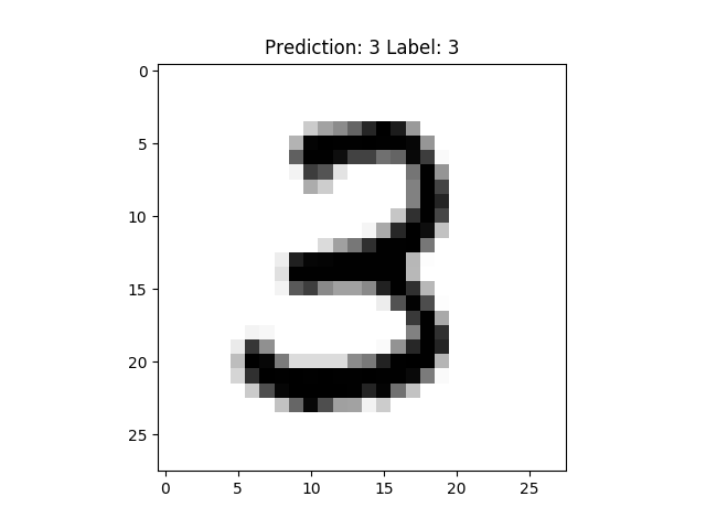After 500 Iterations:

It seems this model can learn perfectly for “3” at 11th position after merely 100 iterations.

Full code can be found here

LSTM (Long-short term memory)

See my next post!

A Few Notes

There is an amazing online course by Stanford that will familiarize you with Tensorflow. The course is called CS20.

You can check out the link here.

Tweet Share